How Far Can You Read a Model From Its Weights?
Four checkpoints, two cheap instruments, and the limits of a zero-data capacity ledger
paper 1 five-seed interventions manuscript in preparation
There is a tempting version of mechanistic interpretability in which the weights tell you everything. Find the crowded directions, the high-gain blocks, the near-duplicates, and you could read a model’s capacity ledger straight from the checkpoint file: no replay data, no gradients, not even a forward pass. If that worked, a continually adapted model could know what not to overwrite simply by inspecting itself.
Paper 1 asks how far that shortcut actually goes. I took the zero-data weight signal into the field and made it compete with two better-informed rivals: a four-minute activation capture, and a gradient-based reference that gets to see the task data. They compete on four operational questions. Which neurons work together? Which ones are risky to update? Which ones mix tasks? Which ones deserve scarce precision?
The answer is useful precisely because it is not clean. The shortcut comes back from the field bruised but alive: one outright win, one demotion to a tradeoff, one firm wall, and one race it loses to a cheaper rival. Where each of those happens is the story of this post.
You do not need to have read anything else here; the next section builds the setup from scratch. This is the blog version of the Paper 1 manuscript while the arXiv submission is being prepared, and it emphasizes the operational picture rather than reproducing the paper section by section.
Code snapshot: the footprint capture, weight-geometry, co-use, sequential-update, census, and quantization pipelines. The mirror now also carries Paper 2’s mechanism code; this post is Paper 1 only.
- A four-minute activation capture per model (the footprint) is stable within a text regime, with centered cosine about 0.99, and identifies the regime from a single sequence at 98-100%. Raw token counts do not reproduce its geometry.
- Neurons whose write directions crowd together really do fire together: crowded pairs co-activate at 1.6-3.5x what independence predicts. But all static weight features combined explain only 3.5-17% of realized co-use.
- On TinyLlama, freezing the most crowded 20% of neurons beats a random mask on both retention and new-task learning, recovering 72.5% of Fisher’s retention benefit with zero task data. The cheap footprint does better still, at 84.4%.
- On Qwen, under a healthy validated protocol, no mask beats random on both axes: more protection means less new-task learning. A frontier, not a continual-learning win.
- Scale does not close the gap. From Qwen2.5 1.5B to 14B, the weight-only signal stays weakly aligned with Fisher.
- The firmest negative: crowding does not rank task-regime mixing (Post 3 has the preregistered null in full). And below four bits of precision, a short activation capture carries information that static weight geometry misses.
The setup, briefly
The cast is four open checkpoints, small enough to dissect on one machine: Qwen2.5-1.5B, Gemma-2-2B, Pythia-1.4B, and TinyLlama-1.1B. Everything here happens in their MLP blocks. Each MLP neuron reads from the residual stream (the vector that flows through the network, accumulating each layer’s contributions), decides how strongly to fire, and writes its contribution back along its write vector: one column of the down-projection matrix, with normalization gain folded in where needed. The write vector is the direction the neuron adds to the stream.
The zero-data instrument is crowding. For each neuron, take its write vector and ask how close it sits to its same-layer neighbours: the largest absolute cosine similarity against any other write vector in the layer. A crowded neuron shares its output direction with a neighbour; an isolated neuron writes somewhere no one else does. Nothing but the checkpoint file enters this number. No examples, no labels, no activations, no gradients.
The cheap usage instrument is the footprint. Run the model briefly over a small corpus spanning five kinds of text, which I will call regimes: math answers, math prose, code, code prose, and ordinary prose. For each neuron, record how often its activation lands in its layer’s top 1% (the 99th percentile, hence q99). Those five firing rates are the neuron’s footprint. The full capture is roughly 375,000 tokens and takes about four minutes per model on the test machine.
The expensive reference is diagonal Fisher information: backward passes on the retained task estimate which parameters the loss is locally sensitive to. It is not ground truth, but it is the data-rich rung that the cheap instruments are trying to approximate.
| rung | needs | what it knows |
|---|---|---|
| weight crowding | checkpoint only | local geometric overlap |
| firing footprint | one short forward capture | distribution-conditioned usage |
| diagonal Fisher | task data + backward passes | local loss sensitivity |
The central mistake to avoid is collapsing these into one concept called “importance.” They measure different things. The experiments ask when those things happen to agree.
First, try to break the instrument
Before trusting footprints to protect or quantize anything, I tried to break them. Split a regime in half and compare the halves: the centered footprint cosine stays near 0.99 at every layer, essentially the resampling noise floor. Compare different regimes instead and the worst layer in each model still clears a three-sigma separation criterion by 31-144x. Shuffle the labels and the margin collapses to zero. The instrument held.
A nearest-centroid classifier identifies the regime from a single sequence’s footprint at 98-100%. That accuracy by itself is not impressive; classifiers built on raw token counts also saturate on these datasets. The more useful test is placement. Plain-English math questions and code descriptions sit closer to their computational siblings in footprint space than token statistics predict, in all four checkpoints, with net swings of +0.16 to +0.75 for math prose and +0.29 to +0.66 for code prose. The footprint knows something the word counts do not.
It is not a pure readout of “computation,” though. The footprint still knows about dataset and register, and footprints taken while the model generates text drift well beyond the reading noise floor, so reading and generation need separate references. The claim is narrower: a tiny forward capture produces stable, useful telemetry that raw token counts do not reproduce.
Trial 1: which neurons work together?
The weight map finds a striking worst case everywhere. Across checkpoints, the 99th percentile of pairwise write overlap is only 0.06-0.17: the bulk of the dictionary looks roomy. Yet the single largest coherence reaches 0.78-1.00. Near-duplicate write directions exist at every depth in every model.
Those overlaps are operational, not decorative. Roughly 500 pairs per layer were stratified by write cosine and checked against real joint activity. Near-orthogonal pairs fire together at or below what independence predicts, with median lift 0.71-1.06. Crowded pairs fire together at 1.6-3.5x independence, and the top decile reaches 7-59x. Training has not quietly arranged overlapping writes so that they take turns.
So the geometry is real. It is just not sufficient. Add reader overlap and base firing rates to build the full static model, and it explains only 3.5-17% of co-use rank variance. Gemma-2 is the most weight-legible case: its reader-set overlap reaches Spearman \rho=0.38 and largely absorbs the incremental geometry term, yet even there the ceiling is 17%. On Qwen, Pythia, and TinyLlama, reader overlap adds little.
One family difference deserves a note. About half the crowded pairs in gated MLPs are anti-parallel opponents (+v and -v), versus 18% in plain-GELU Pythia. Simultaneous overlap is real; whether it is redundancy, cancellation, or harmful interference cannot be read from an absolute cosine alone.
Trial 2: which neurons are risky to update?
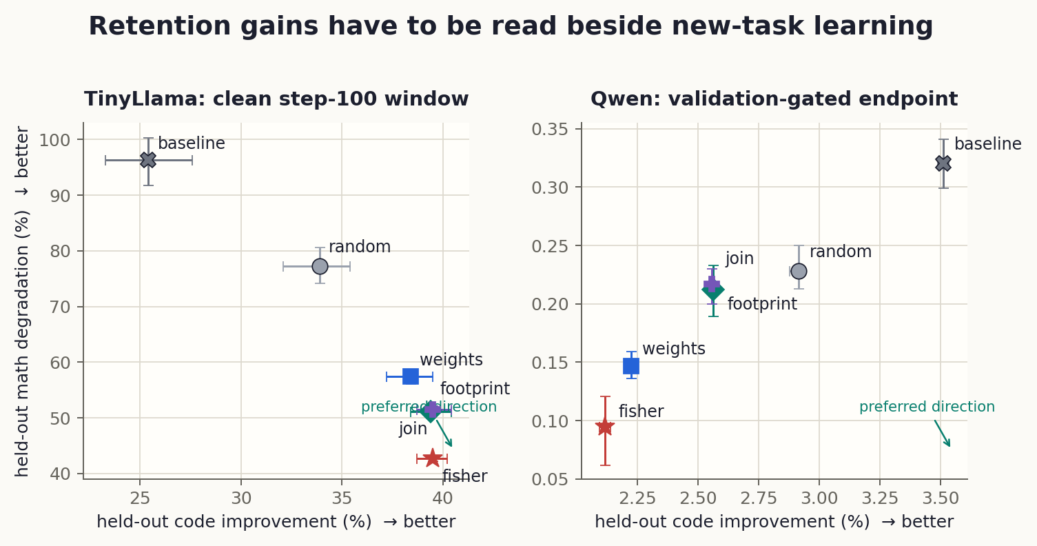
Correlation is cheap, so the centerpiece is causal. Every arm starts from the same checkpoint that has just learned math, then trains its MLP weights on code. Before the code training begins, 20% of neurons per layer are frozen according to one rule: none, random, weight crowding, math footprint, crowding times footprint, or Fisher. The zero- and low-data masks are captured at the base checkpoint and stay fixed. Only Fisher is computed after math.
Both outcomes are reported, because either one alone can lie. Less math degradation means better retention; more held-out code improvement (code the model never trained on) means better acquisition. Calling a mask good because it forgets less, while hiding that it also learns less, would bury the central tradeoff.
TinyLlama: the shortcut’s best day
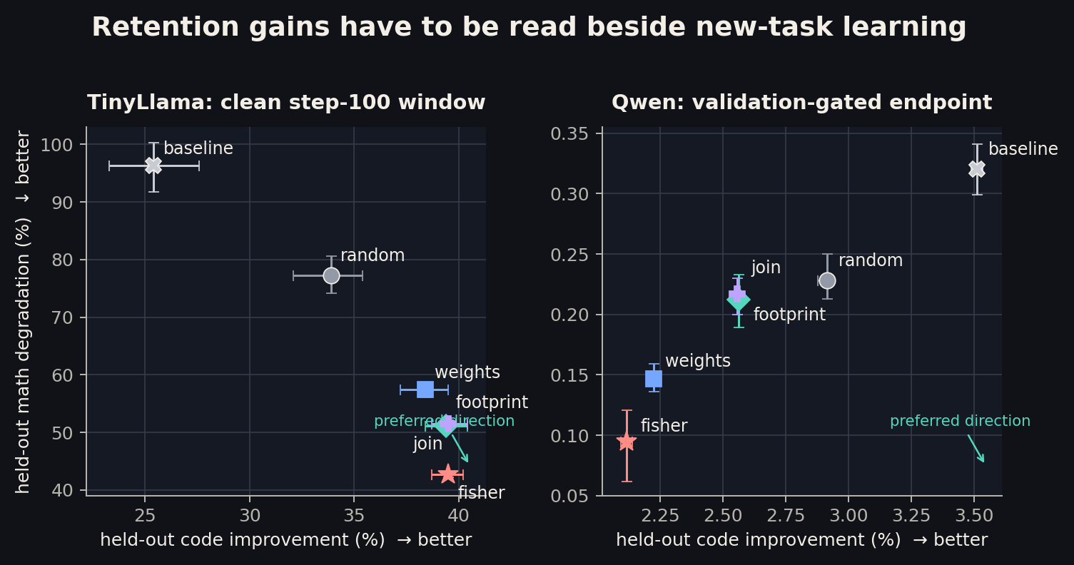
At step 100, before repeated passes over the small code corpus begin to overfit, every arm improves held-out code. And here all four informed selectors beat the equal-budget random mask on both axes at once.
| arm | math degradation | code change | Fisher retention recovered |
|---|---|---|---|
| Fisher | +42.7% | −39.5% | 100.0% |
| footprint | +51.1% | −39.4% | 84.4% |
| join | +51.5% | −39.5% | 83.6% |
| weights | +57.4% | −38.4% | 72.5% |
| random | +77.3% | −33.9% | 35.2% |
| baseline | +96.3% | −25.4% | 0.0% |
The weight-only mask cuts math degradation by 20.0 percentage points relative to random while improving code by another 4.5 points. Across five phase-B data-order seeds it recovers 72.5% [70.7, 74.3] of Fisher’s retention benefit, without ever seeing a single token of task data. The forward-only footprint is stronger still at 84.4% and nearly matches Fisher on code learning.
That is the clean positive result. Raw geometry contains an intervention-relevant signal, and cheap usage adds more.
Qwen: the complication
The first Qwen schedule was too aggressive. Held-out code worsened from the first evaluation in every arm, which means the impressive-looking mask ranking it produced was only a damage stress test, not evidence of continual learning. I repaired the protocol before looking at any protected-arm endpoints: a frozen train/validation split, a tenfold lower learning rate, and validation-selected checkpoints within fixed budgets. Both the math acquisition gate and the phase-B code gate passed.
Under that healthy protocol, every arm learns code, and none of the informed masks is Pareto-superior to random. The weight-only mask reduces math degradation from 0.228% to 0.147%, but gives up 0.689 points of code improvement. Fisher retains best and learns least. The unprotected baseline learns most and forgets most.
The honest reading is a stability-plasticity frontier, not a win. Fixed-step retention alone cannot distinguish “protected old knowledge” from “the optimizer was prevented from learning as much.” A matched-update or matched-acquisition design would be needed to make the stronger claim.
Does scale rescue the shortcut?
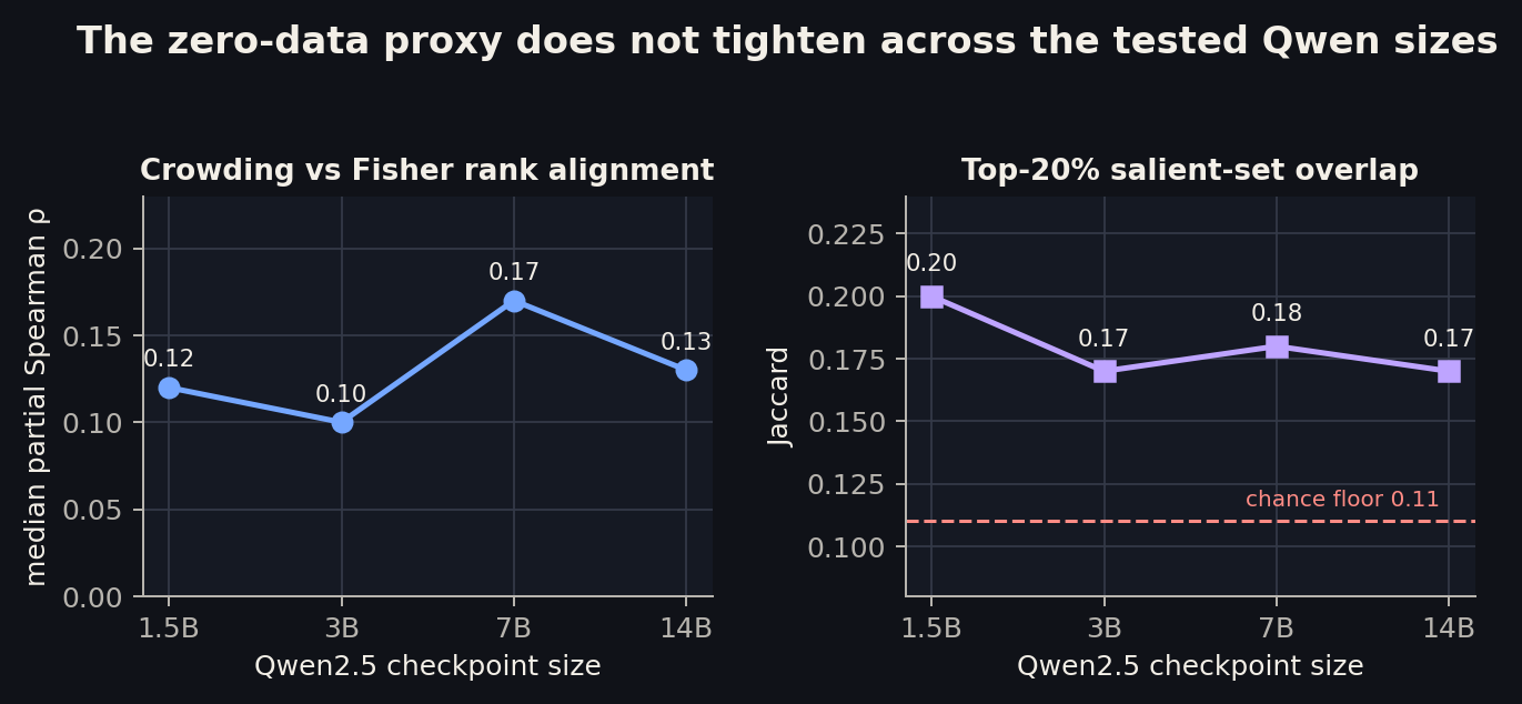
Perhaps geometry is merely noisy at 1-2B parameters and becomes Fisher-like in larger models. Across the tested Qwen2.5 series, it does not. The median rank agreement between crowding and Fisher is +0.12, +0.10, +0.17, +0.13 at 1.5B, 3B, 7B, and 14B. The top-20% salient-set overlap stays at 0.17-0.20, only modestly above the 0.11 chance floor.
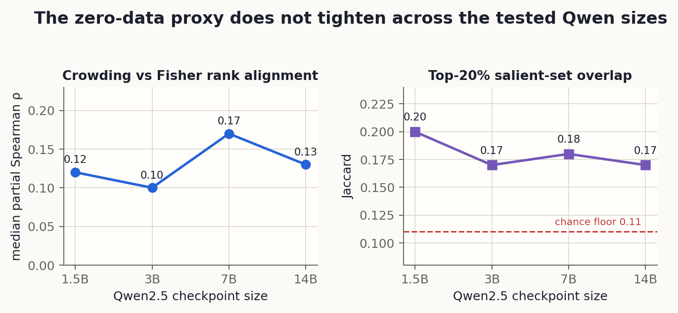
Under the fixed stress protocol, weight-only recovery falls from 90% at Qwen 1.5B to about 20% at 3B, and at 7B the baseline and Fisher arms barely separate, so the recovery ratio is not identifiable there. This is not a scaling law; the effective update and task competence are not matched across sizes. But it is clear evidence against the hopeful claim that the proxy gap closes over the tested range.
Trial 3: which neurons mix tasks?
This trial ends at a wall, and the wall is the program’s firmest fact. It gets only a summary here because Post 3 reports it in full. Neuron crowding does not provide a practically useful rank of task-regime mixing on either MLP interface in any checkpoint: all eight primary measurements sit inside the pre-registered |\rho|<0.10 null band.
The pipeline itself is not to blame. The same code recovers a planted law at +0.52, and its entropy proxy tracks known mixing in a trained toy model at +0.83. The null is about the world, not the instrument. Weight geometry can predict an intervention without yielding a semantic atlas.
Trial 4: which neurons deserve scarce precision?
Quantization supplies a different actuator and a useful consistency check. Keep every weight at four bits, then give eight bits to the top 1% of neurons under each signal. Random protection recovers nothing. Usage and gradient signals recover 47-85% of the four-bit damage. And because quantization noise is not conditioned on any task, the footprint gets promoted here: it recovers about 85% of the gap on TinyLlama and can match or beat the gradient-guided rung on these checkpoints.
With sequential GPTQ (a standard error-correcting quantizer), the ranking is nearly saturated at four bits; every rung lands within 0.16 perplexity. Differences emerge at three bits and below, where activation energy recovers 55%, 12%, and 19% of the three-bit damage at Qwen2.5 1.5B, 3B, and 7B. None of this is a new quantizer. It is a practical hint: when the precision budget is genuinely tight, a short activation capture carries information that static weight geometry misses.
The ledger after contact with data
The zero-data dream does not survive intact. It does not collapse either.
Weight geometry comes out of the trials as a prior, not a verdict. It locates crowded writes, predicts elevated co-use, and produces a causally useful protection mask in one clean checkpoint. It does not replace observed usage or loss sensitivity, and it does not read task semantics at all. The footprint, meanwhile, turns out to be an unusually good middle rung: stable, distribution-conditioned, cheap enough to refresh, and often competitive with gradient-based signals whenever the intervention depends on usage magnitude.
The Qwen repair is the part I would most want a practitioner to carry away. Pair every retention number with an acquisition number, because protection that merely stops the optimizer from learning is not protection. The repair changed the story from “geometry protects” to “geometry moves the operating point along a frontier.” That is still useful. It is a different claim.
And heterogeneity is the rule, not the exception. Gemma-2 is unusually weight-legible, TinyLlama gives the clean Pareto result, Qwen gives a frontier. Architecture, scale, tokenizer, and training recipe are all confounded across these checkpoints, so none of this is a family law.
The practical design I carry forward is a two-signal ledger: use the weights as the always-available structural prior, calibrate them with a small footprint captured in the execution mode you care about, and escalate to gradients only when the decision is important enough to pay for them.
One question survives every trial untouched. Why does crowding help at all? A signal that has never seen a token somehow points at the neurons the next task will damage, and nothing in Paper 1 explains that. The trials narrow the possibilities; they do not settle the mechanism. That question belongs to Paper 2, and to a later post.