A Weight-Space Map of Attention Heads in Gemma-2 (with SAEs)
Lab notes on mechanistic interpretability without activations
partially retracted → corrected see the errata post (2026-06-14)
This post uses model weights plus a fixed SAE feature basis to map what kinds of routing and writing patterns are available inside Gemma-2 attention heads. The emphasis is on available linear structure in a shared feature coordinate system, not on claiming that a head uses that structure on typical tokens.
The payoff is a depth-wise map of head behavior without collecting new activations or running generation for the main analysis. That map makes it possible to ask a narrower question than “what does this head do?”: what kinds of computations do the weights make available here, and where do those capabilities concentrate with depth?
This is a map-making exercise with explicit measurement objects and clear failure modes, not a causal claim. Sign and task relevance still require experiments, which is why the later causal section is a preview.
Code – snapshot of the analysis pipeline accompanying this post.
After publishing, I found three pipeline bugs – RMSNorm gamma folding (missing the +1), the RoPE pairing convention, and validating against the wrong (post-layernorm) activations. After fixing them and re-running, two headline claims on this page do not hold:
- The late-layer “anti-predictive regime” (Regime 3) was an artifact. Every layer is solidly predictive once the bugs are fixed (grand-mean Spearman \rho rises from +0.011 to +0.229, every layer positive). There is no anti-predictive regime.
- The unique Layer-6 selectivity spike is overstated – the spike survives but L8/L12/L14/L22 share the band, and the identity-routing peak is actually at L10.
The Layer-23 causal result still replicates, but its explanation changes. The corrected map, two new studies (an SAE-checkpoint diagnostic at L13 and a dictionary-free dual-basis comparison), and the full numbers are in the follow-up: Correcting the Weight-Space Map. The body below is left as originally published for the record.
- We map 200 attention heads (layers 1–25 of Gemma-2-2B) using weight-space analysis with SAE decoder directions – no activations required.
- Weight-space maps are reliable in early/mid layers (local \rho up to 0.82, 144/200 heads show local structure), but become anti-predictive in late layers (mean \rho = -0.14 after L17). The overall mean \rho = 0.07 averages out this sign flip.
- Layer 6 shows an extreme selectivity spike (105\times uniform baseline) – two orders of magnitude above other layers.
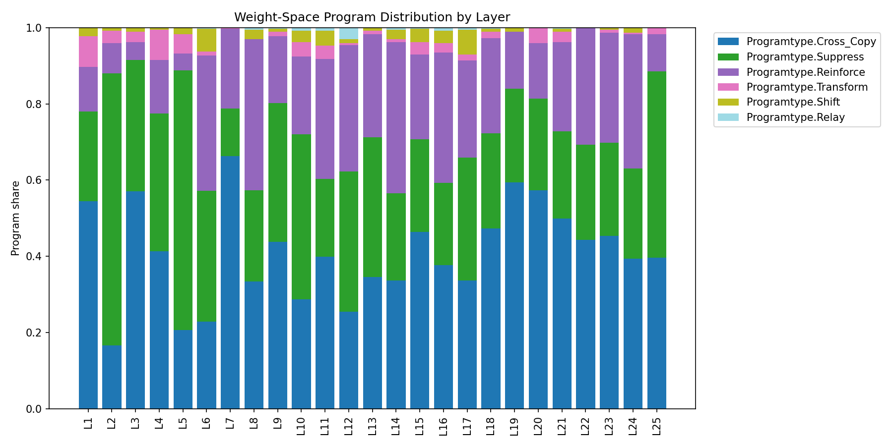
- Depth-dependent program shifts: early layers carry high SUPPRESS share alongside CROSS_COPY (filtering-like), mid layers mix CROSS_COPY/SUPPRESS/REINFORCE (composing-like), late layers lean CROSS_COPY (propagating-like).
- Long-range routing structure weakens but persists: 114/200 heads clear |\rho| \geq 0.10 at 128–256 tokens, 108/200 at 256+.
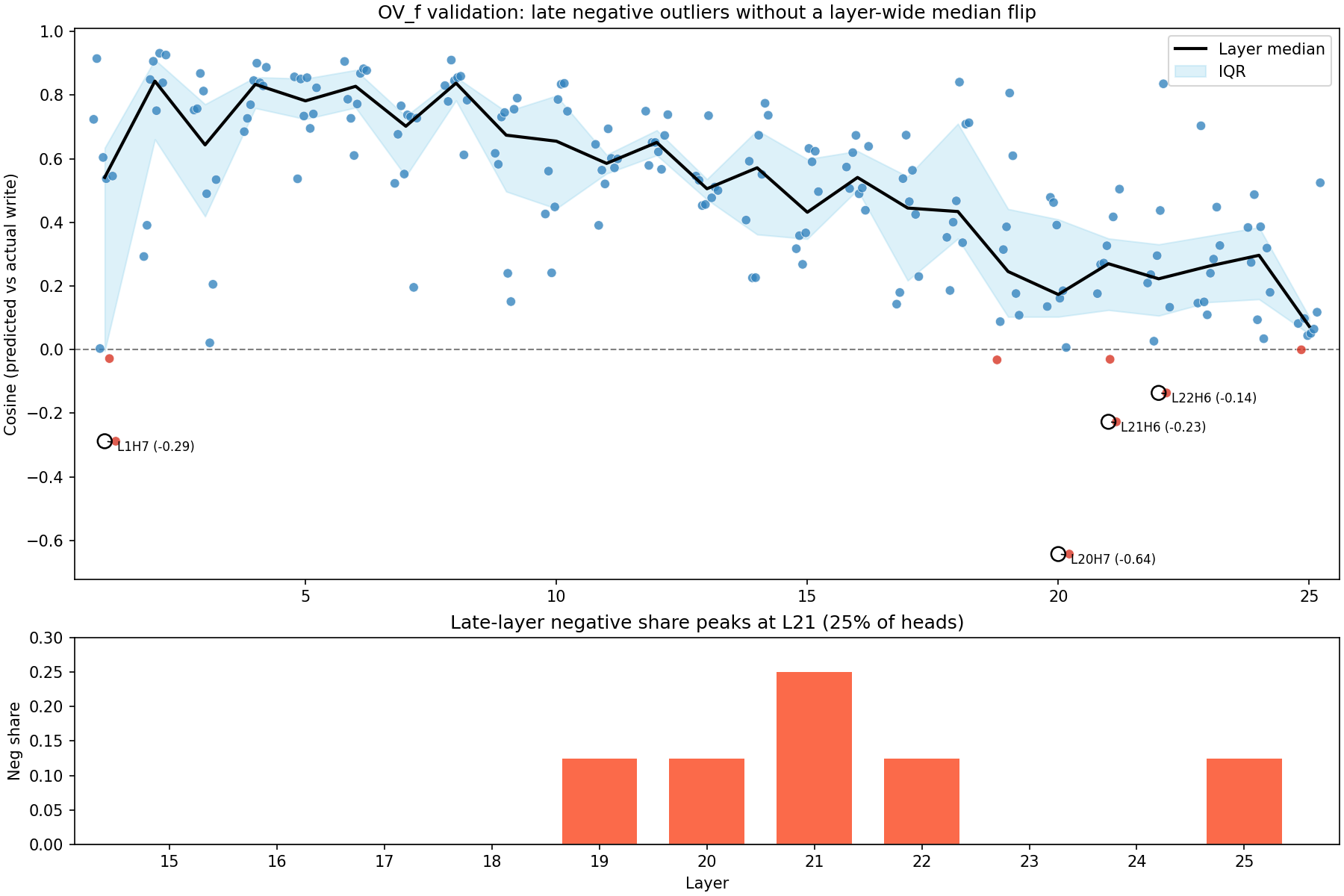
- OV negatives are late-layer outliers, not a layer-wide flip; strongest outlier is L20H7 at -0.64.
- Causal preview: ablating Layer 23 heads improved retrieval accuracy by +8.7% – the map identified a high-leverage layer, but not the sign of its behavioral effect. Full results in Post 2.
The post builds three measurement objects (QK routing, OV writing, feature programs) and validates them against activations. The punchline is that depth organizes attention into three regimes:
- Early layers (L1–L5): feature transport and filtering – modest selectivity, validated routing, SUPPRESS-heavy programs.
- Mid layers (L6–L12): a routing bottleneck – selectivity spikes (Layer 6 at 105\times baseline), the map is most predictive here, strongest validation-confirmed heads cluster.
- Late layers (L17+): the map becomes anti-predictive at runtime (\rho flips negative) – still shows structure in weights, but the fixed SAE basis stops being a reliable behavioral proxy.
The sections below build up to this picture. If you want the conclusion first, jump to Three Depth Regimes.
Setup
We use the base model Gemma-2-2B (26 layers).
It uses Grouped Query Attention (GQA): 8 query heads and 4 KV heads, so each KV head is shared by 2 query heads. This means each query head has its own output projection (W_O) but reads from a shared value signal (W_V). We analyze query heads (not KV heads), since each has its own routing and writing behavior.
One implication is worth keeping in mind later: sister query heads share the same value source but can still look very different in the map. When that happens, the specialization is unlikely to come from W_V alone; it has to be coming from routing (W_Q/W_K), the per-head output projection (W_O), or both.
Gemma-2 scales attention logits by \text{query\_pre\_attn\_scalar}^{-1/2}. With
query_pre_attn_scalar= 256, we have s = \sqrt{\frac{1}{256}} = \frac{1}{16} = 0.0625.Softcap value: c = 50.0.
Gemma-2 uses sliding window attention in alternating layers starting at index 0: even layers are sliding-window with size 4096, odd layers are global (full causal attention up to the model’s max context length, 8192 tokens).
To talk about “features” rather than neurons, I use Google’s Gemma Scope Sparse Autoencoders (SAEs). SAEs decompose model activations into sparse, interpretable directions. Each learned “feature” is a direction in residual-stream space that tends to activate for a coherent pattern. This gives us a model-aligned coordinate system for analyzing attention: instead of asking “which neuron fires?”, we can ask “which interpretable feature does this head route or write?” These SAEs are trained on base Gemma-2 models.
Analysis choice: I use the SAEs trained at the “Residual SAE” tap point. Attention in block L consumes the residual stream produced by block L-1. Thus, in my runs I use an SAE layer offset (-1) so the SAE basis matches what the attention block actually sees. Each SAE feature has a decoder direction (a vector in residual space). I’ll treat those decoder directions as a convenient, model-aligned basis for analysis. Please note that SAE decoder directions are not orthogonal and activations are nonnegative.
For details on the available SAEs, see Google’s Gemma Scope documentation.
Throughout, I fold the learned RMSNorm scale (\gamma) into weights but ignore the token-dependent normalization factor (1/\|x\|_{\text{RMS}}). This makes the analysis strictly linear-in-direction rather than exact-in-activation. The approximation is tighter when the residual stream has stable norms (early/mid layers) and more suspect in layers with high statistical heterogeneity – which may partly explain the late-layer degradation discussed later.
Using the base model avoids instruction-tuning artifacts and keeps the focus on the raw attention mechanism.
The main weight-space metrics (selectivity, program distribution, write archetypes) use a 4,096-feature random subset of the 16,384 SAE features for computational tractability. Qualitative patterns are stable across seeds. The activation validation run (Sanity Check section) uses the full 16,384-feature set with RoPE-aware affinity matrices. When absolute numbers differ between sections, this is usually why.
Weight-Space Object #1: Content-Only Routing in Feature Space
For a single attention head, I want a matrix that answers:
“If the query looks like feature i, which key-feature j does this head prefer?”
Let:
D be the SAE decoder matrix for a subset of features (shape n \times d_{\text{model}}), one row per feature direction. (Convention: I treat decoder directions as row vectors; if you store decoders as columns, transpose accordingly.)
W_{Q}, W_{K} be the head’s query/key projection matrices
Project decoder directions into Q-space and K-space:
Q_f = D \cdot W_Q^T
K_f = D \cdot W_K^T
Define the content-only affinity matrix (what attention logits would look like if RoPE and masking weren’t present):
B = (Q_f \cdot K_f^T) \cdot s
Where s = \sqrt{\frac{1}{256}} = \frac{1}{16} = 0.0625 (Gemma-2’s attention logit scaling).
Gemma-2 also applies a tanh soft-cap to attention logits; when matching the model’s behavior, I apply the same cap:
\text{softcap}(x) = c \cdot \tanh\left(\frac{x}{c}\right)
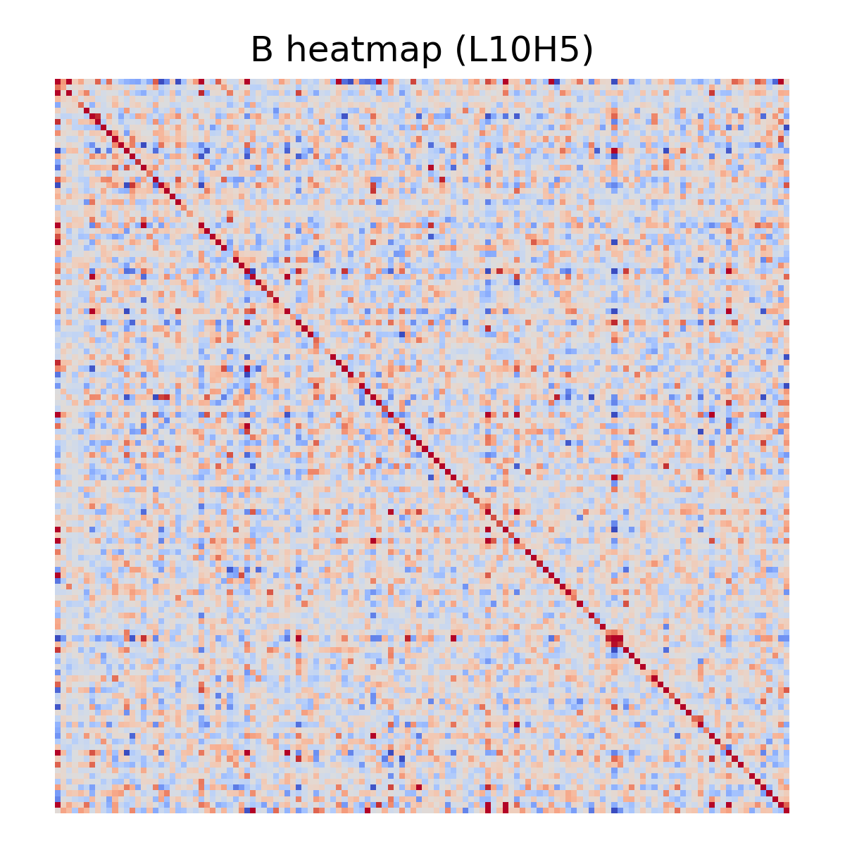
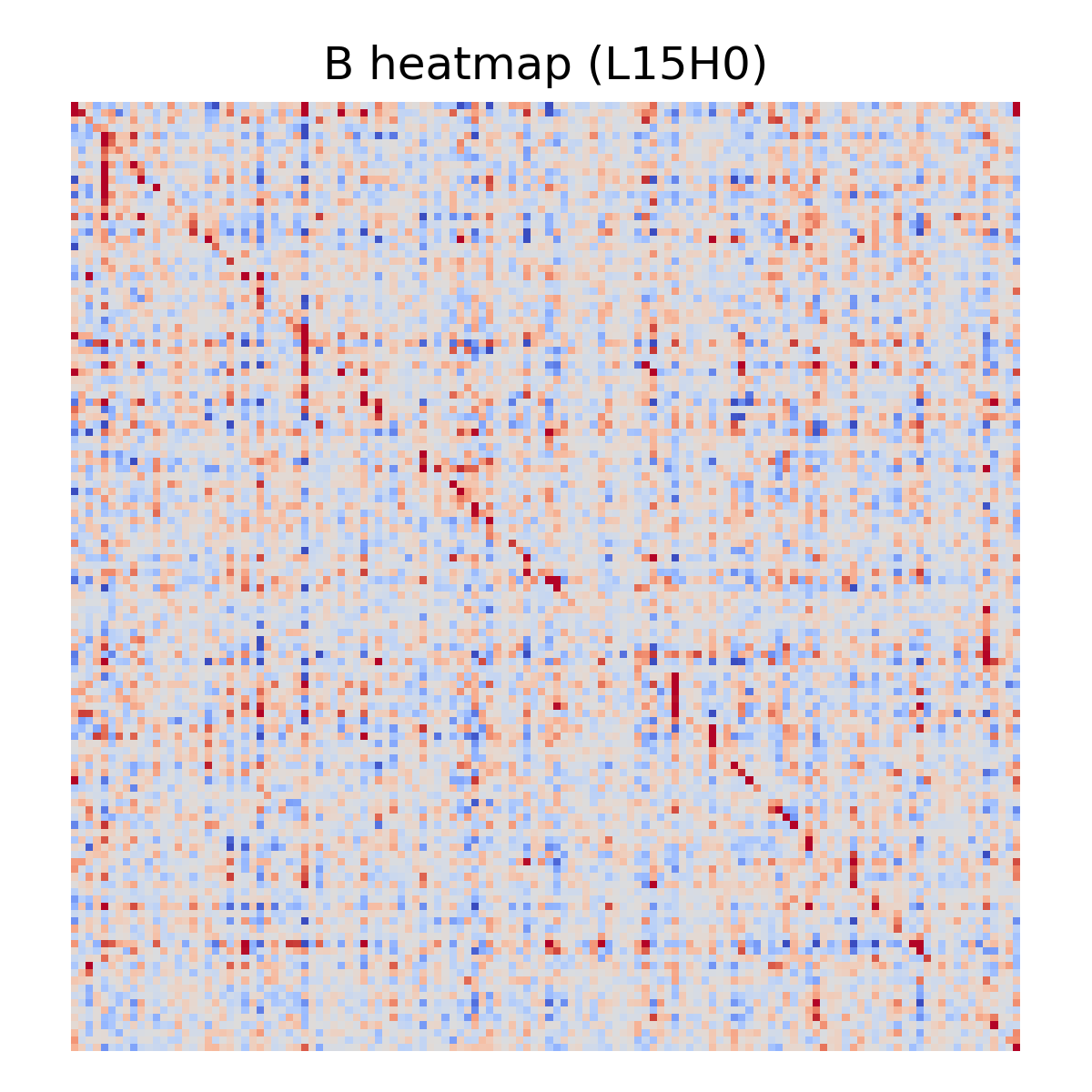
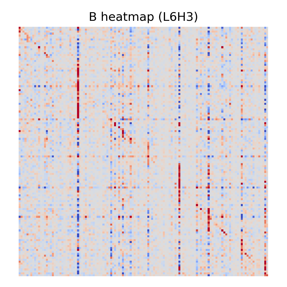
This B matrix is the backbone of our routing analysis. From B we can define simple, interpretable routing metrics:
Selectivity (peakiness): per row i, softmax over keys and take max probability; average over i – “top-1 softmax mass”
Identity sensitivity: how much softmax probability lands on the diagonal entry (i attends to i) – “diagonal softmax mass”
Max-gap: difference between best key score and runner-up (in logits), averaged over rows
Avoidance: Negative entries in B indicate low dot-product affinity. I treat extreme negative tails as a signature of selective exclusion, but it’s not the same thing as suppression unless the OV path also writes negative feature directions.
Important: rows/cols of B are SAE features, not tokens. When I compute “top-1 softmax mass”, the softmax is over key features j, not over token positions.
A few examples:
Sanity Check: Does B Predict Real Attention Routing?
Although the map in this post is computed purely from weights plus a fixed SAE basis, I ran an activation-grounding sanity check to confirm that the main routing object (the feature affinity matrix B) predicts runtime attention patterns.
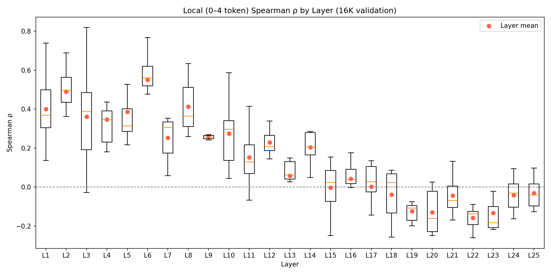
Across 200 heads (25 layers x 8 heads), using all 16,384 SAE features and RoPE-aware affinity matrices B_\Delta, the activation-grounding run covers about 4.45M token pairs per head. The headline result is mixed in exactly the way that turned out to matter for interpretation: the map is usefully predictive in early and mid layers, but degrades sharply in late layers. The layerwise spread and threshold counts are shown in Figure 4 and Figure 5.
For ~25 diverse prompts, I captured the pre-attention residual stream at the target layer, encoded it into the same SAE feature subset used in the weight-space map, and predicted attention preferences using the bilinear form a(t)^T B\, a(s). For the runtime target, I used log attention weights. I compute correlations per query row and then average (to avoid cross-row normalization artifacts), and I also break correlations out by distance bins; log-softmax equals logits up to a per-row constant, so rank correlation is meaningful even though each row has its own normalization.
To account for RoPE, I also computed RoPE-aware affinity matrices B_\Delta per distance bin by rotating K (\Delta set to the bin center) and applying Gemma’s tanh softcap, then compared predicted vs runtime attention within each distance bin.
Summary statistics for the same run:
- ~4.5M token pairs per head
- Mean overall Spearman \rho = 0.07 (std=0.21)
- Mean local (0–4 tokens) Spearman \rho = 0.15 (max=0.82)
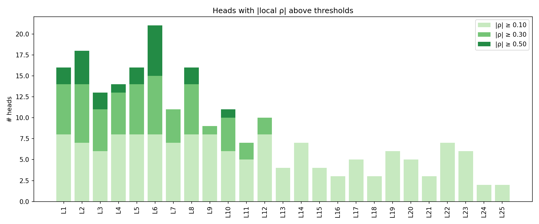
- 144 heads (72%) show |\text{local } \rho| > 0.1 (‘structured’ routing)
- Best local correlation: L5H4 with \rho = 0.82
- Best overall correlation: L6H4 with \rho = 0.57
The important caveat is that correlation is not uniform across depth. In early layers (L1–L5), 35 of 40 heads show positive overall Spearman \rho (mean +0.16), and mid layers (L6–L12) are even stronger (47/56 positive, mean +0.22). But in late layers (L19–L25), 50 of 56 heads show negative overall Spearman (mean -0.14), meaning the weight-space B matrix predicts the opposite of the observed attention pattern. This degradation likely reflects nonlinear interactions or representational drift that are not captured by the linear SAE decomposition. My best guess is that the fixed residual-stream feature basis becomes a poorer proxy for the computation actually being deployed near the top of the network, where the model is closer to logits and late residual mixing is more consequential. That is an interpretation, not a demonstrated mechanism. The weight-space map remains a useful guide in early/mid layers but should be treated as a capacity map rather than a behavior map past roughly Layer 17.
The distribution is heavy-tailed: many heads are near-zero (diffuse), while a smaller set shows strong, structured routing (e.g., best local \rho = 0.82). The top 10 heads by overall Spearman (L6H4, L5H4, L3H2, L6H3, L8H1, L8H0, L6H2, L8H6, L12H3, L12H2; all \rho > 0.45) cluster in layers 3–12.
Please note that this doesn’t prove any head is causally responsible for a behavior; it just checks that the measurement objects used in the map are anchored to runtime attention.
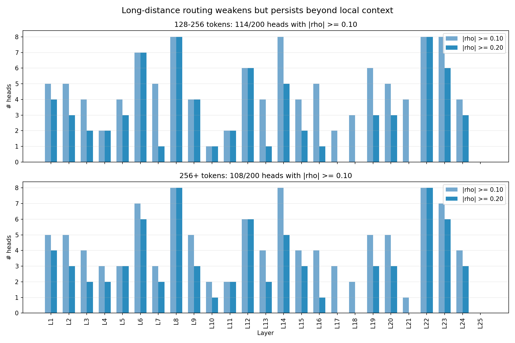
Long-range structure is weaker than local routing, but it is not absent. At 128–256 tokens, 114/200 heads still clear |\rho| \geq 0.10, and 108/200 do so at 256+; the more important failure mode is the late-layer sign reversal in overall routing correlations rather than a complete disappearance of long-range structure.
Baselines: What Counts as “Real Structure”?
Softmax selectivity is extremely sensitive to logit scale, so we need baselines that match the right thing. I use three baselines, each designed to kill a different kind of structure:
Random decoder directions (random D): Replace decoder directions with random unit vectors (matched norms), keeping W_Q/W_K fixed
Random weights baseline: Replace W_Q and W_K with random matrices (same shape), then rescale B to match \text{std}(B) before computing softmax-derived metrics. Specifically, we rescale B_{\text{baseline}} \leftarrow B_{\text{baseline}} \times (\sigma_{\text{real}} / \sigma_{\text{baseline}}), where \sigma = \text{std}(B).
Permuted-K baseline: Shuffle key-feature identities by permuting rows of K_f (equivalently, permuting columns of B), so diagonal mass becomes ‘chance self-match’.
This lets me say things like:
“Selectivity is X times the random-weights baseline.”
“Diagonal mass is X times the permuted-K baseline.”
Why both matter:
top-1 mass is permutation-invariant (it only cares that you pick something)
diagonal mass is identity-sensitive (it cares that you pick self)
Weight-Space Object #2: What a Head Writes (OV) in Feature Space
Routing is only half the story. Even if a head can attend cleanly, it only matters if its output projection writes a direction that’s salient in the SAE feature basis into the residual stream.
For a query head, its write is determined by:
W_V for the KV group (shared across 2 query heads in Gemma-2 GQA implementation)
W_O for the specific query head
Gemma’s effective OV matrix is implemented as (row-vector convention; W_O is [d_\text{model} \times d_\text{head}], W_V is [d_\text{head} \times d_\text{model}]):
W_{OV} = W_O \cdot W_V
For each SAE feature direction d_j (row of D), define the write vector:
\text{write}_j = d_j \cdot W_V^T \cdot W_O^T
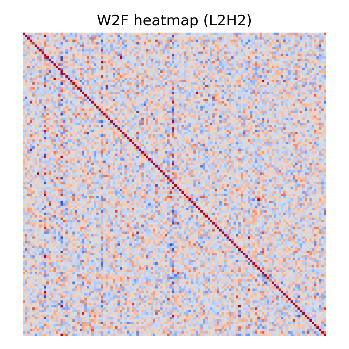
Project write vectors back onto decoder directions to get a “write-to-feature” matrix:
\text{W2F}[j,k] = \cos(\text{write}_j,\, d_k)
Note: W2F uses cosine similarity, so it measures directional alignment and discards magnitude; later I’ll also report write norms / activation-grounded deltas so ‘aligned-but-tiny’ writes don’t get over-interpreted.
This helps us define archetypes with concrete scoring.
With W2F as the cosine similarity matrix between each feature’s write vector and all decoder directions, we define:
COPY score = mean(diag(W2F)): how much feature i writes back to itself
TRANSFORM score = max off-diagonal of W2F: strength of the strongest i \to j\neqi mapping
BROADCAST score = max column sum of W2F: how many features write to the same target
SUPPRESS score = |min off-diagonal of W2F|: strength of the most negative write
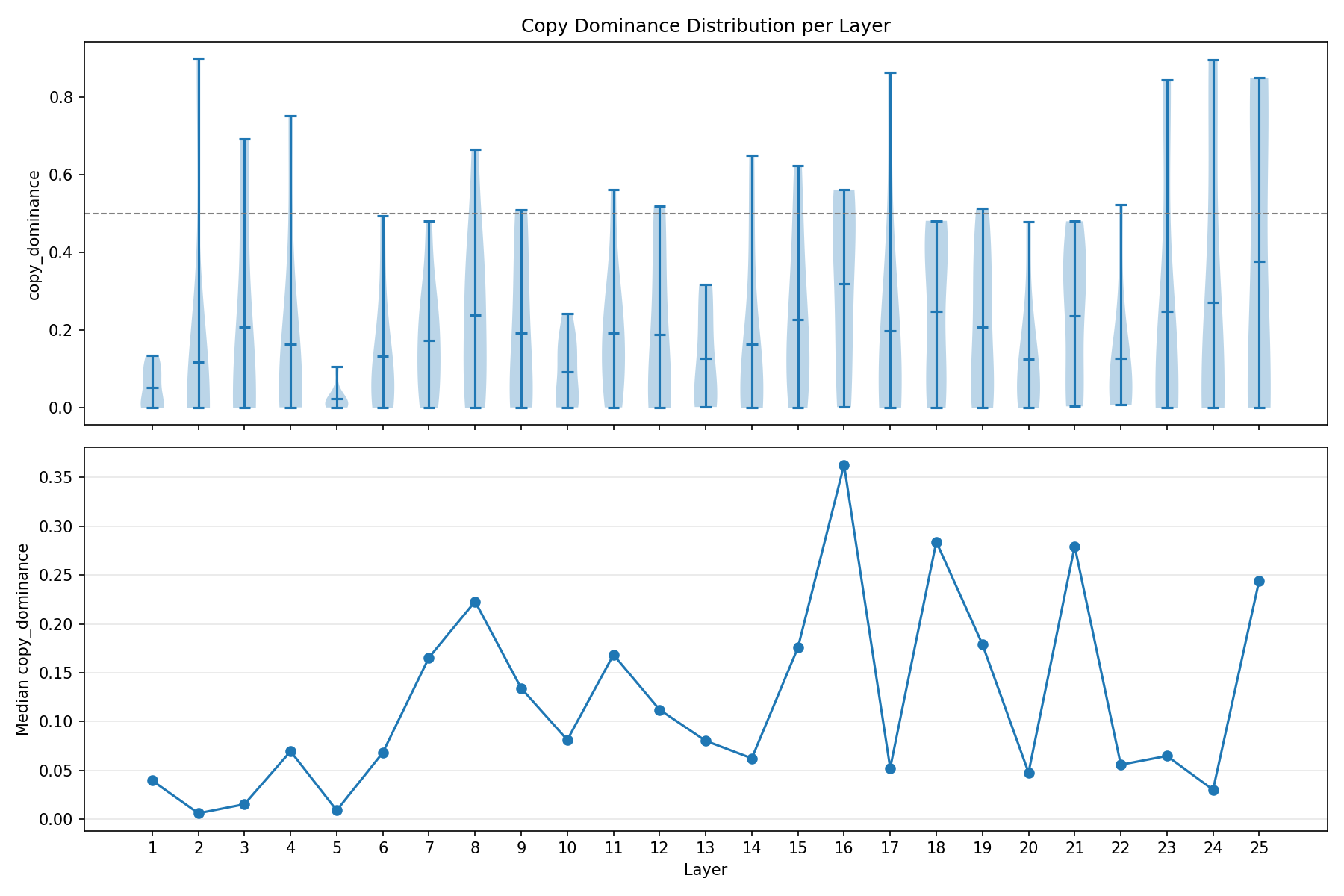
Copy dominance remains low on average (mean 0.186), but the more informative pattern is the upper tail: the strongest copy head is the early outlier L2H2 (0.897), while a secondary cluster of near-copy heads appears in L23–L25. The distribution by layer is shown in Figure 7.
A head is classified by whichever score crosses its threshold first (COPY > 0.3, TRANSFORM > 0.5, BROADCAST > 3x copy, SUPPRESS > 0.5), defaulting to DIFFUSE (no score crosses any threshold). I assign a single label using a precedence rule (COPY \to TRANSFORM \to BROADCAST \to SUPPRESS \to DIFFUSE). Heads can score highly on multiple axes; the label is just meant to be a coarse summary. These thresholds are heuristic cutoffs chosen to separate tails in this run, not a claim that the taxonomy has canonical boundaries.
In this taxonomy, SUPPRESS means the head routes positively to some key feature j, and then the OV write is negatively aligned with a target feature k (it is not about negative B/avoidance). Also, please note that COPY can be negative if the head writes anti-aligned to the feature’s decoder direction.
A few examples:
OV validation shows a different failure mode from QK routing: late layers develop negative outliers, but not a layer-wide median inversion. Most late-layer medians stay positive, yet a subset of heads flips sign, peaking at 25% negative heads in L21; the strongest outlier is L20H7 at cosine = -0.64.
Weight-Space Object #3: Composing “Feature Programs” (i \to j \to k)
Once we have routing (B) and writing (W2F), we can compose them into simple “programs”:
query feature i \to attend key feature j \to write feature k
Programs are extracted from the top tail of routing scores and write scores (quantile thresholds), so the taxonomy describes high-confidence motifs rather than all mass. We also track when a self-write is a fallback rather than a measured OV target.
Each triplet is scored by combining route strength and write strength. Then we can classify it into a small motif family:
| Type | Flow |
|---|---|
| REINFORCE | i \to i \to i |
| SHIFT | i \to i \to k (k \neq i) |
| CROSS_COPY | i \to j \to j (i \neq j) |
| RELAY | i \to j \to i (i \neq j) |
| TRANSFORM | i \to j \to k (all different) |
| SUPPRESS | i \to j \to -k |
This is the point where the analysis becomes human-legible: you can say “this head’s weight structure is consistent with CROSS_COPY” or “this layer is SUPPRESS-heavy in the weight-space taxonomy,” without running a prompt.
In my run: routing tail \approx top 10%; write tail \approx top 20%.
When a routing pair (i\toj) passes the route threshold but has no explicit write evidence, the system can inject a synthetic self-write using the head’s copy_score as a fallback. This means some REINFORCE programs may be artifacts of missing write evidence rather than genuine self-reinforcing circuits. The explicit-only program histogram (without fallbacks) is more conservative and should be preferred for circuit-level claims.
Position Robustness: RoPE Stability
Gemma-2 uses RoPE, which rotates Q/K vectors as a function of relative position. In weight space you can simulate this by rotating keys (or queries) and recomputing affinity matrices.
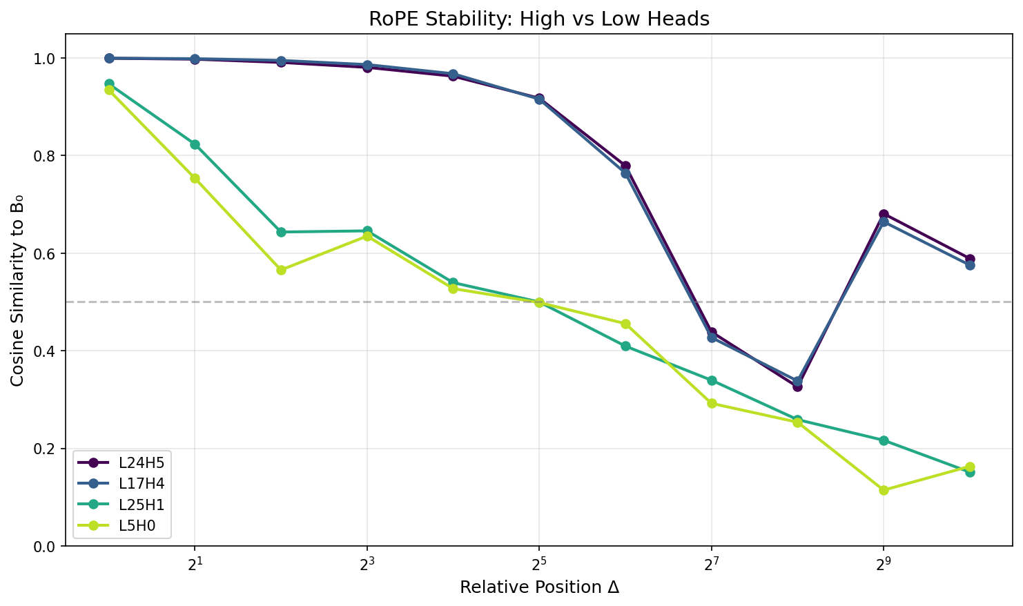
Let B_0 be affinity at relative offset \Delta=0, and B_\Delta at offset \Delta. Define a stability score (e.g., cosine similarity of flattened matrices):
\text{stability}(\Delta) = \cos(\text{vec}(B_0),\, \text{vec}(B_\Delta))
Then compress the curve across \Delta into a single number (AUC-style over log-distance). I call this RoPE stability: a summary of how similar the affinity matrix B stays as we apply relative-position rotations. Also, we apply the tanh softcap before comparing matrices.
When this metric is High \to routing seems to be mostly content-controlled and stays similar across positions. It could also mean that this head doesn’t use positional information much because it’s doing something else entirely.
And when it is Low \to routing depends strongly on relative position (more “twitchy”).
This is not “style steerability,” but it is a useful proxy for “position-invariant content routing.”
One caveat: cosine similarity can look high if B is very low-magnitude / diffuse; I interpret stability alongside routing strength/selectivity.
Results: What Changes with Depth?
Once we compute these objects across layers and heads, we can summarize how the model’s attention machinery evolves with depth.
1. Local (Sliding-Window) vs Global Layers
Gemma-2 alternates local and global attention by layer, giving a built-in contrast:
Sliding-window layers can’t directly attend to tokens outside the window, but they can still transform a residual stream that already contains long-range information injected by earlier global layers.
Global layers are the only layers that can implement direct long-range attention pointers.
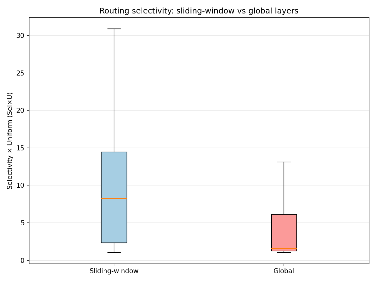
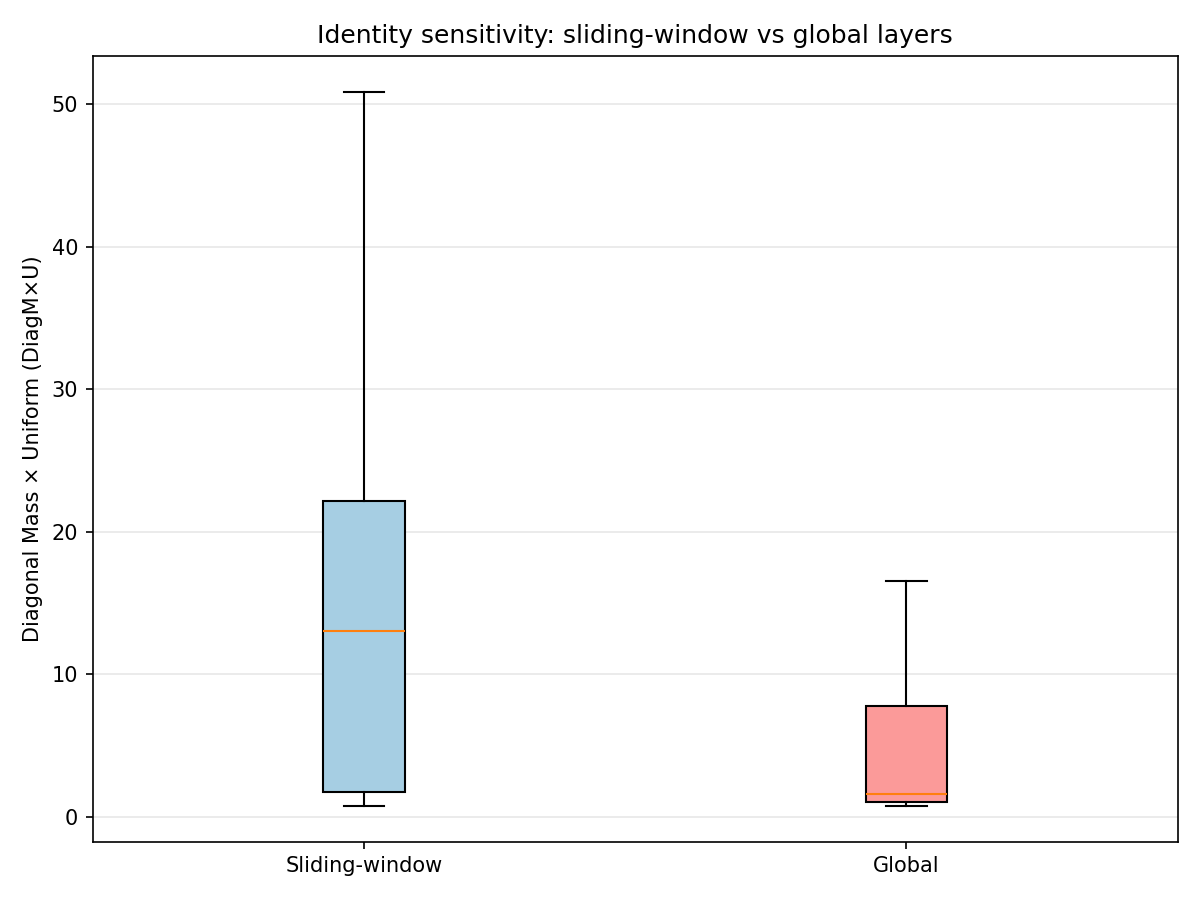
2. Selectivity and Identity-Sensitivity Are Not Monotone
Two different things can happen as depth grows:
Peakiness (top-1 softmax mass) can increase because the model learns sharper “addressing”
Identity sensitivity (diagonal softmax mass) can increase if heads learn an i\toi “feature self-match” pattern
In my current run, there’s a very strong spike in these metrics around a mid layer (one layer stands out dramatically on both selectivity and diagonal mass). That suggests a “band” of unusually crisp routing behavior rather than a smooth trend.
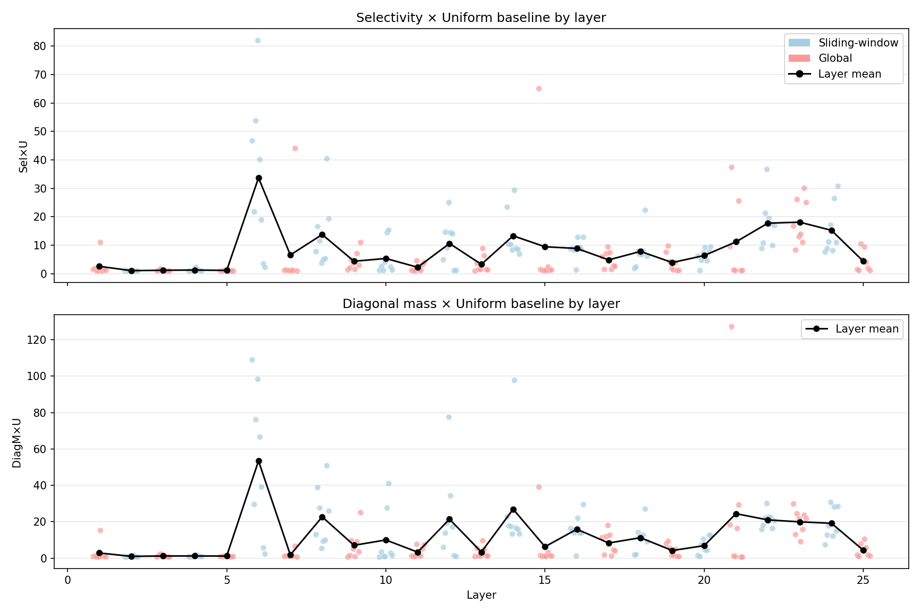
The Layer 6 spike was the single most dramatic finding – Sel\timesU of 105 means the routing structure is two orders of magnitude above uniform baseline. I expected a smooth gradient, not a spike. This showed up consistently across different feature subsets and seeds. Layer 6 is a sliding-window layer (even index) in the range where induction-like heads are typically found, and four of its heads (L6H0, L6H2, L6H3, L6H4) are among the top-10 validation-confirmed heads. The spike-rather-than-gradient pattern suggests a sharp regime change in routing behavior at this depth.
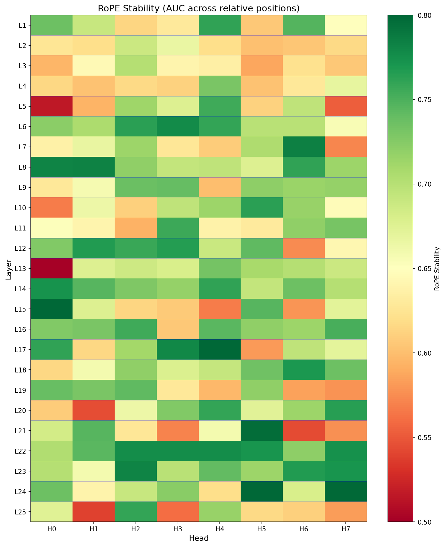
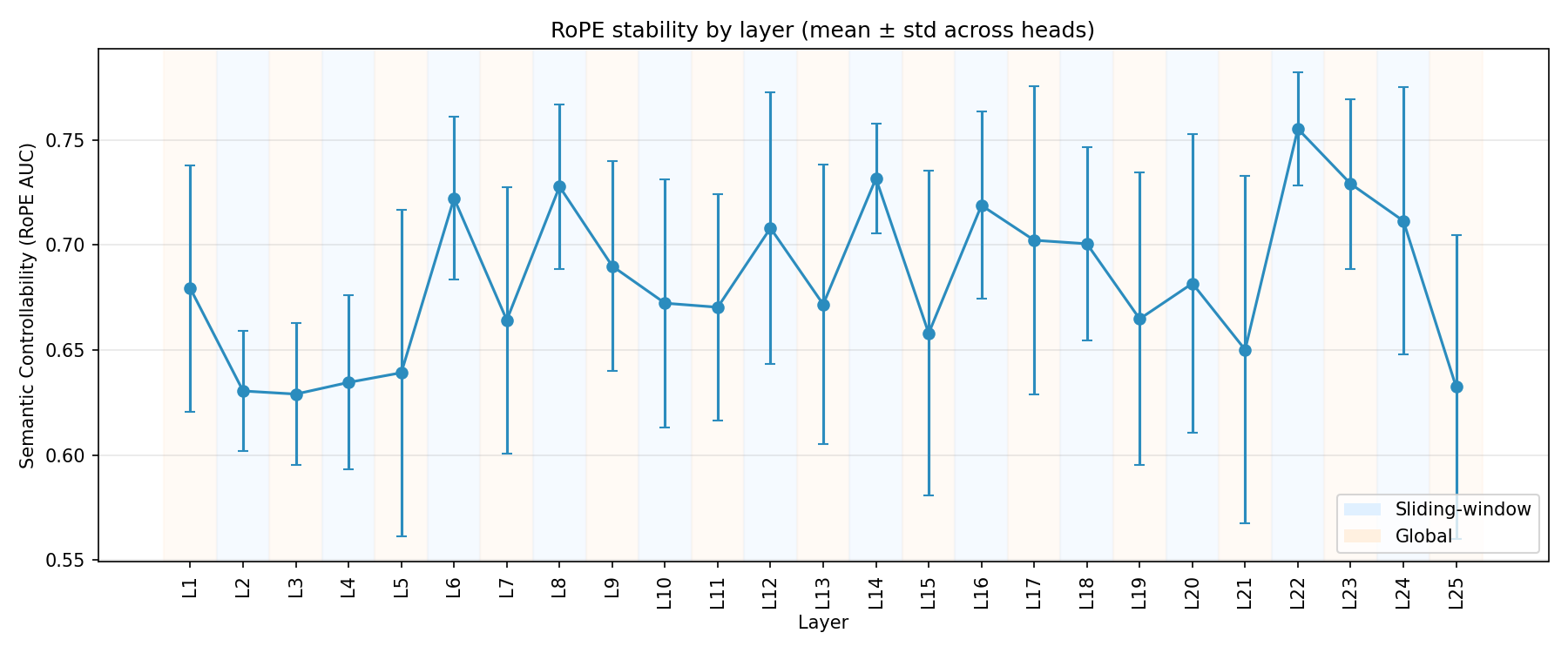
3. RoPE Stability Tends to Rise with Depth (with Bands)
RoPE stability tends to increase with depth, but it’s not smooth. There are high-stability bands (mid layers and a late cluster near the top of the network).
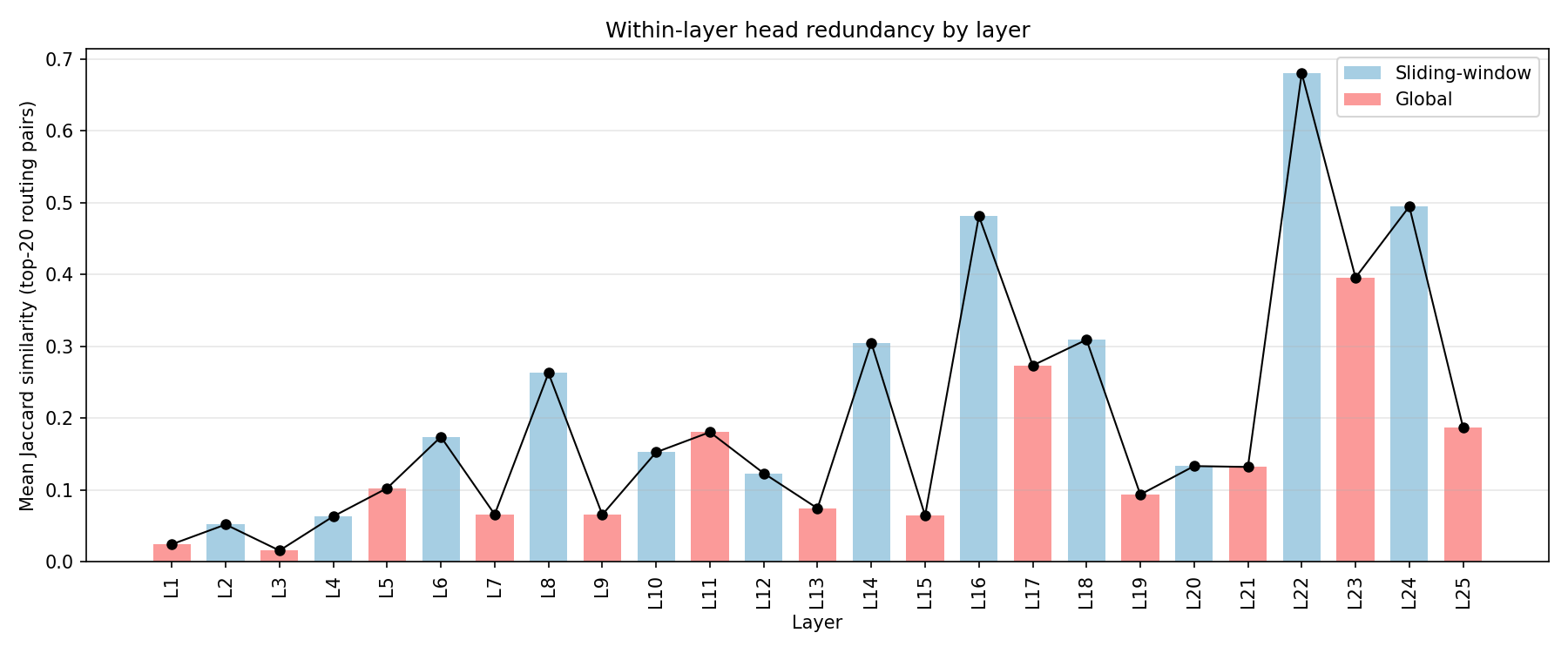
4. Redundancy vs Uniqueness (Where Structure Concentrates)
I track how redundant heads are within a layer (do they “do the same thing” in program space?). Redundancy = Jaccard similarity of top-20 routing pairs between heads – that is, |A \cap B| / |A \cup B| where A and B are each head’s set of top-20 (query \to key) feature pairs. Two heads are considered redundant if they route the same feature pairs highly:
Low redundancy: a few specialized heads carry most structure – could be potential larger single-head “levers”
High redundancy: many heads share similar top programs – could mean that the layer is robust to removing any one head
To avoid noise, I primarily interpret redundancy within the subset of heads that show structured routing (e.g., above a small selectivity or correlation threshold).
Working Interpretation: Three Depth Regimes
Taken together, the plots suggest a cleaner story than any single metric does on its own:
Early layers mostly look like feature transport and filtering. Routing is validated, selectivity is modest, and OV behavior is often suppressive or transform-light.
Mid layers, especially the Layer 6 band, look like a routing bottleneck. This is where the map is most predictive, selectivity spikes, identity-sensitive routing appears crisply, and several of the strongest validation-confirmed heads cluster.
Late layers still show strong structure in the map, but the QK side becomes anti-predictive at runtime. The natural reading is not “late layers are uninterpretable”; it is “late layers are where this fixed linear feature basis stops being a reliable behavioral proxy.”
I think this is the most important qualitative insight in the post. The headline is not just that certain layers spike, but that the kind of structure the map is surfacing changes with depth.
The program distribution by layer (Figure 19) makes this concrete: early layers carry substantial SUPPRESS (peaking in L2/L4–L6) alongside CROSS_COPY, mid layers mix CROSS_COPY / SUPPRESS / REINFORCE, and late layers tilt toward CROSS_COPY. The dominant program motif changes with depth even when the global histogram looks stable.
Interpretation
Weight-space analysis is not telling you “what the model will output.” It’s telling you what kinds of operations are available in the weights, and where in depth those operations concentrate.
Safest takeaways from this weight-space + SAE-basis analysis:
Local vs global layers are qualitatively different substrates. If a behavior requires long-range access, only global layers can implement it directly.
There are depth bands with unusually crisp routing (spikes in selectivity and sometimes identity-sensitive diagonal mass).
Redundancy varies a lot. Some layers look like “few special heads,” others spread structure across many heads.
Intervention heuristic: Combining selectivity (0.3 weight), RoPE stability (0.4), head diversity (0.2), and max-gap (0.1) into a composite score, Layer 6 emerges as the strongest routing intervention candidate (score 0.51), followed by Layers 22–23. I now view this as a prioritization heuristic rather than a steering claim: the Layer 23 ablation result shows the map can identify leverage without predicting direction of effect.
Behavioral Follow-Up: Predictions and Early Results
Pre-Registered Expectations
In Post 2, I will test behavior, but driven by pre-registered weight-space predictions.
One candidate hypothesis: heads with high selectivity and strong directional write structure (high COPY/TRANSFORM/etc scores) but low RoPE stability could contribute disproportionately to long-distance errors on retrieval-style tasks; ablating their OV contribution may measurably change accuracy (possibly improve or worsen), especially at large distances.
What Already Came Back
I ran causal ablation experiments on Layer 23 – which the weight-space map flagged as a high-selectivity, high-RoPE-stability late layer – ablating individual heads and multi-head combinations on retrieval-style prompts with symmetry controls (swapped A\leftrightarrowB) and logits-only evaluation (no generation artifacts).
The surprising result: ablating 6 of 8 Layer 23 heads (H0, H1, H2, H3, H6, H7) improved retrieval accuracy from 58% to 66.7% (+8.7%) and widened the logprob margin from +0.34 to +0.59. H4 and H5 were excluded because their individual ablation reduced accuracy. The weight-space map correctly identified L23 as a high-leverage layer, but the direction of effect was opposite to the naive prediction – these heads appear to interfere with correct retrieval rather than facilitate it. Whether this reflects genuine suppressive behavior or a limitation in the task design is an open question for Post 2.
I also ran a full OV writing validation across all 200 heads confirming that predicted feature writes match actual head output with mean cosine similarity of +0.50 in early/mid layers, but develop negative outliers in late layers – not a layer-wide median inversion. Most late-layer medians stay positive, yet a subset of heads flips sign, peaking at 25% negative heads in L21; the strongest outlier is L20H7 at cosine = -0.64 (see Figure 11). This finding persists with the full 16K feature set. Post 2 is in preparation.
Implementation detail note: model constants like attention scaling, RoPE placement, and alternating sliding-window convention are codified in the project config.
This work is inspired by Anthropic’s Transformer Circuits series, especially A Mathematical Framework for Transformer Circuits.
Code for the analysis pipeline is available in the code/weight-space-map directory of this site’s repository (experimental research code snapshot).
Feedback, comments, and discussion are welcome.
Limitations
Linearity assumption. We fold RMSNorm \gamma into weights but ignore the token-dependent 1/\|x\|_{\text{RMS}} factor, making the analysis linear-in-direction rather than exact-in-activation. This approximation is tighter when residual stream norms are stable (early/mid layers) and degrades where norm variance is high (late layers). This is likely one contributor to the late-layer anti-prediction effect.
SAE basis is not ground truth. SAE decoder directions are non-orthogonal and learned via reconstruction loss – they may not capture the model’s “true” features. Feature splitting (one concept spread across multiple SAE features) and superposition (multiple concepts encoded in one direction) can distort the affinity matrix B. We do not apply Gram-matrix correction for superposition in the main analysis, though the infrastructure exists.
Late-layer anti-prediction. After ~Layer 17, the weight-space B matrix predicts the opposite of observed attention (mean Spearman \rho = -0.14). This is not just noise – it’s systematic. All late-layer metrics (selectivity, program distribution, write archetypes) should be interpreted as “what the weights make available” rather than “what happens at runtime.” The sign flip likely reflects LayerNorm interactions, residual stream composition, or accumulated superposition that the linear analysis cannot capture.
Feature-space selectivity \neq token-space selectivity. A head can have diffuse routing over SAE features while being sharp over token positions, or vice versa. Our selectivity metrics measure peakiness in feature space – this is a different (though correlated) quantity from attention sharpness over positions.
No direct causality. Weight-space analysis maps available operations, not actual behavior. A head scored as high-COPY might never copy in practice because it never receives the right input distribution. Causal validation (ablation, activation patching) is required to make functional claims – which is why Post 2 is in preparation.
Single-seed sensitivity. As noted in the Feature Subset Note above, the main weight-space metrics use a 4,096-feature random subset. Absolute values (e.g., exact Sel\timesU numbers) shift across seeds. Qualitative patterns (which layers spike, program distribution shape) are stable in spot checks but have not been formally assessed for robustness.
Appendix: Metric Glossary
top1_mass = mean over query features of max softmax probability across keys
Sel\timesU = top1_mass \div (1/n)
diagonal_softmax_mass = mean softmax mass on the diagonal entry (identity-sensitive)
DiagM\timesU = diagonal_softmax_mass \div (1/n)
MaxGap = average(top1_logit - top2_logit) per row
RoPE (stability) = AUC summary of how stable B remains under RoPE-relative rotations (called
semantic_controllabilityin the code)Copy = mean diagonal of W2F (self-write strength)
Trans (transform) = max off-diagonal of W2F (strongest i \to j\neqi mapping)
COPY / TRANSFORM / BROADCAST / SUPPRESS / DIFFUSE = write archetypes derived from W2F. DIFFUSE = no score crosses any threshold
Feature programs = composed triplets i \to j \to k with a small taxonomy