Why Crowding Protects
Four suspects, one mechanism: a second-order detective story
paper 2 preregistered manuscript in preparation
Train a language model on something new and it quietly gets worse at things it already knew. This is catastrophic forgetting, and one blunt but effective defense is to freeze a fraction of the network while the new training runs. The interesting question is which fraction.
In an earlier study I found something that kept bothering me. You can pick the neurons to freeze using no data at all: just look at the weight file, find the neurons whose output directions crowd together, and protect those. On the model where the protocol is cleanest, that zero-data mask recovered most of the benefit of the expensive, gradient-based alternative. A signal that has never seen a task, a token, or a gradient somehow knows which neurons the next task will damage.
That should strike you as suspicious. Geometry does not know what the model was trained on. Why would it know what is fragile?
This post is the answer, run as a detective story, because that is how the investigation actually unfolded: four natural explanations, each eliminated by a preregistered test, and then a mechanism that survives everything we could throw at it. You do not need to have read the earlier posts; the next section rebuilds the setup from scratch.
Code and provenance. Every experiment here was preregistered before running, with amendments dated and disclosed, on a frozen git history with a SHA256 manifest of all result artifacts. The mechanism code is public: the curvature probes and sketches, the K2 selector, the interface decomposition, both isolation controls, the rollback surgery, and the reparameterization self-test, alongside the training and analysis code they build on. The preregistration trail and result artifacts ship with the Paper 2 manuscript, which is in preparation.
- Forgetting damage is a second-order phenomenon: at the end of training on a task, gradients are nearly flat, so damage arrives through the loss’s curvature, and specifically through cross-neuron (off-diagonal) curvature coupling.
- Crowded neuron pairs carry 6.1x the coupling of orthogonal pairs matched on rate, gradient size, weight norm, update size, and co-firing, in 16 of 16 measured layers. After normalizing away self-curvature the contrast is still 5.1x: the effect is genuinely between neurons, not within them.
- The coupling’s anatomy matches the algebra that predicts it: 81% flows through read-side changes emitted along existing aligned write vectors, and the only pathway gated by raw co-activation carries 3%, which is why co-firing tests come up empty.
- Measuring the coupling directly (a quantity we call K2) yields the best retention selector observed in the program: better than crowding by a wide margin and better than Fisher on 6/6 seeds (exact p = 0.0156).
- The value is off-diagonal specifically: with self-curvature, first-order alignment, Fisher, crowding, and movement all matched (and audited), high- coupling neurons undo 77% of damage when restored; matched low-coupling neurons undo 18%, less than random’s 32%.
- The account predicts its own boundary: rescale the network in function-preserving ways and protection value swings wildly, because curvature lives in the optimizer’s coordinates. Real fine-tuning holds the parameterization fixed, so the ledger applies there.
The setup, briefly
Everything happens in the MLP blocks of a small language model (TinyLlama-1.1B). Each MLP neuron reads from the residual stream (the vector that flows through the network, accumulating each layer’s contributions), decides how strongly to fire, and then writes its contribution back through its write vector: one column of the down-projection matrix. The write vector is the neuron’s handwriting, the direction it adds to the stream.
Crowding is a property you can compute from the weight file alone: for each neuron, take the largest absolute cosine similarity between its write vector and any other write vector in the same layer. A crowded neuron shares its output direction with a neighbor. An isolated neuron writes somewhere no one else does.
The experiment that produced the mystery is a two-phase curriculum. Phase A teaches the model math. Phase B trains it on code, and math quietly degrades. Before phase B starts, we freeze the top 20% of neurons per layer according to some signal, and afterwards we measure how much held-out math was lost (as negative log-likelihood, NLL: lower degradation is better). The candidate signals form a cost ladder:
| signal | needs | what it measures |
|---|---|---|
| crowding | the checkpoint only | write-direction overlap |
| footprint | one short forward capture | how often each neuron fires on math |
| Fisher | task data + backward passes | local loss sensitivity |
The Paper 1 field report established that every informed mask beats a random one here, and that crowding, the bottom rung, recovers 72.5% of Fisher’s retention benefit with zero data. (There is also a firm negative: crowding does not predict which neurons mix tasks semantically. That boundary got its own post.) What Paper 1 could not say is why the cheapest signal works. Time to interrogate suspects.
Suspect 1: a tug-of-war between tasks
The most intuitive story: crowded neurons are where the two tasks fight. If math and code both use a shared direction, their gradients should pull it in conflicting ways, and protecting the battleground prevents the damage.
This is directly measurable: correlate each neuron’s crowding with the misalignment between task gradients (the cosine between its math gradient and its code gradient, negated so that bigger means more conflict). Across three models the correlation is -0.001, -0.043, -0.020. Nothing. Crowded neurons are not gradient battlegrounds. The first-order tug-of-war does not exist at the neuron level, let alone explain the protection.
Suspect 2: crowding is secretly Fisher
Maybe geometry is just a blurry photocopy of loss sensitivity: crowded neurons are important neurons, and we have merely rediscovered Fisher information at a discount.
If so, the two signals should rank neurons similarly. They do not. Rank alignment between crowding and Fisher sits between 0.1 and 0.36 depending on the checkpoint, and the top-20% masks they select overlap barely above the chance floor. Crowding protects while disagreeing with Fisher about which neurons matter. Whatever it knows, it is not a cheap Fisher estimate.
Suspect 3: standing in the optimizer’s path
Perhaps crowded neurons are simply where phase B writes its update. Protection would then be trivial: freeze the neurons the optimizer was about to bulldoze.
Correlationally, crowding barely tracks movement (about -0.05 on TinyLlama). But the causal test is better, and it is the most instructive elimination in the program. After phase B finishes, take the damaged model and surgically restore 20% of neurons to their pre-B values (a “rollback”), choosing the neurons by different signals, and see how much math comes back. Restoring the 20% that moved most brings back about 52% of the lost math; crowding brings back 67%; Fisher 75%; a random set, 27%. Movement is the worst informed selector. The damage does not live where B wrote. It lives where the signals that know something about task A point, and crowding is one of those signals.
Suspect 4: fire together, forget together
The last natural story: crowded neurons co-activate. If two neurons fire on the same tokens, an update that damages one context damages both, and their joint usage is the transmission channel.
We measured co-firing directly (how often both neurons cross their layer’s 99th-percentile activation threshold together, relative to independence) and tested whether it carries or gates the damage-relevant quantity. It does not: in a regression with geometry, co-firing and its interaction with geometry are both null (interaction permutation p = 0.67), and within every geometry stratum co-firing is inert. In case the threshold was the problem, we re-ran the test with continuous co-activation statistics. Null again. Whatever links crowded pairs, it is not that they fire at the same time.
The turn: forgetting is a second-order crime
Here is the reframe that cracks the case. At the end of phase A, training has converged: the gradient of the math loss is nearly flat. To first order, nothing can hurt the model. The damage from phase B’s update \delta\theta arrives through the second-order term,
\Delta L_A \;\approx\; \tfrac{1}{2}\, \delta\theta^\top H_A\, \delta\theta,
where H_A is the curvature (Hessian) of the math loss. Curvature is a matrix over pairs of parameters, and that plural is the whole point. Its diagonal blocks are self-curvature: how sensitive the loss is to moving one neuron alone, which is roughly what Fisher tracks. Its off-diagonal blocks are coupling: whether moving neuron j changes the price of having moved neuron i. If a pair couples positively, updating both together hurts more than the sum of updating each alone. Forgetting, in this frame, is not a list of individually fragile neurons. It has cross terms.
Work out what that coupling looks like for two MLP neurons (using the Gauss-Newton form of the curvature, the positive-semidefinite part that comes from the network’s output geometry), and the dominant term factorizes:
S_{ij} \;\sim\; \underbrace{(w_i \cdot w_j)}_{\text{geometry clock}} \;\times\; \underbrace{\textstyle\sum_t m_t\, c_i(x_t)\, c_j(x_t)}_{\text{usage clock}}
The first factor is the overlap of the two neurons’ existing write vectors, which is exactly what crowding measures. The second is the co-response of their activation changes under the update: not whether they fire together, but whether the update moves their firing together, weighted by how much the output cares. Two clocks, one geometric and one usage-driven, multiplied.
If this account is right, crowding works because it is the zero-data shadow of the geometry clock: it reads one factor of the off-diagonal curvature straight from the checkpoint. And the account makes predictions sharp enough to falsify. Crowded pairs should carry outsized coupling at matched everything else. The coupling should flow through the existing write vectors, not through co-activation. Measuring the coupling directly should beat every proxy of it, including Fisher. And the advantage should survive matching on every diagonal quantity. All four were registered before the tests ran.
Exhibit A: crowded pairs carry the coupling
Measuring off-diagonal curvature naively is hopeless (the matrix is billions-by-billions), so the estimator probes it: perturb one neuron’s parameters along its actual phase-B update direction, and read out how the curvature responds at every other neuron in the layer. Three forward passes and one backward pass per probe, validated against an exact reference implementation on a small oracle model, plus a seven-gate sanity battery. We ran 1,200 probes.
Then the matched contrast: take crowded pairs and orthogonal pairs that agree on firing rate, gradient magnitude, weight norm, update norm, and co-firing (202 matched contrasts), and compare their coupling.
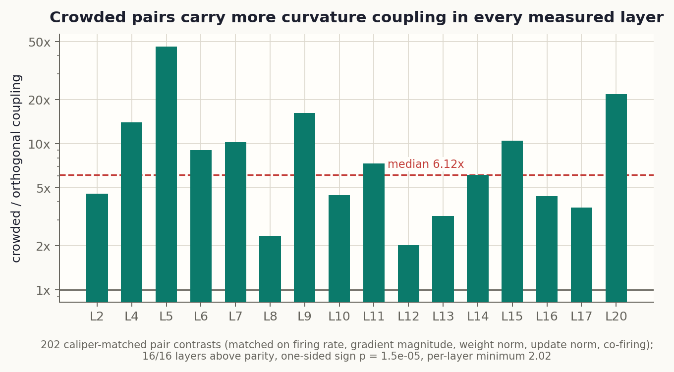
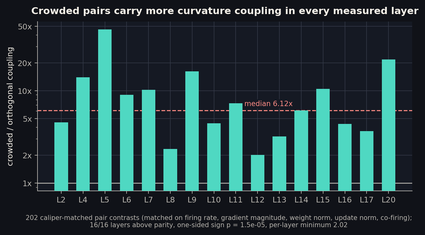
The median crowded pair carries 6.12x the coupling of its matched orthogonal counterpart, and every one of the 16 measured layers shows the effect. The obvious deflationary reading, that crowded neurons just have more curvature of every kind, fails: normalize each pair’s coupling by its members’ self-curvature and the contrast is still 5.06x. The excess is genuinely between the neurons.
Two more registered checks. Crowding correlates with a neuron’s total within-layer coupling load at +0.32, passing the registered bar; the same correlation against a global load that includes cross-layer terms drops to +0.18, a registered miss we report as found. Crowding is a within-layer statistic and sees within-layer load. And the coupling is polarity-blind: pairs whose write vectors point in opposite directions couple exactly like aligned ones (both predominantly positive, 69% and 71%). That refuted our own registered sign prediction, and it vindicates the convention of measuring crowding with absolute cosines: opponent neurons interfere like duplicates.
Exhibit B: the anatomy matches the algebra
The two-clock factorization makes a structural claim: the coupling should be carried by read-side activation changes emitted along the existing write vectors (the w_i \cdot w_j terms), not by update-write overlap gated by co-activation. That is checkable, because each pair’s coupling can be decomposed into blocks by which interface sends and which receives.
On the 50 registered validation pairs, the read-by-read block flowing through base write vectors carries a median 0.812 of each pair’s coupling mass (95% CI [0.737, 0.855]), and no single pair drives the result. The one block that raw co-activation actually gates is the smallest of all nine, at 0.031. This is why Suspect 4 walked free: the tests were correct, and the channel they tested barely exists.
Better, the decomposition contains its own discriminating prediction. The base-write terms scale with w_i \cdot w_j, so read-side dominance should be a property of crowded pairs specifically. It is: median share 0.872 for crowded pairs, dissolving to 0.437 for orthogonal ones. The algebra predicted a fingerprint and the data shows that fingerprint.
Exhibit C: measure the coupling and it beats everything
If off-diagonal curvature is the mechanism, then the mechanism quantity should be a better protection signal than any of its proxies. So we built one: K2, each neuron’s off-diagonal curvature row load along the actual update directions, estimated with randomized sketches. K2 needs one sacrificial unprotected run of phase B to know the update directions; it then selects the top 20% per layer, and we re-run protection with that mask on fresh data seeds. Evaluation is leakage-clean: K2 was built on one half of the held-out math set, outcomes are scored on the other half, and the mask transfers across update seeds.
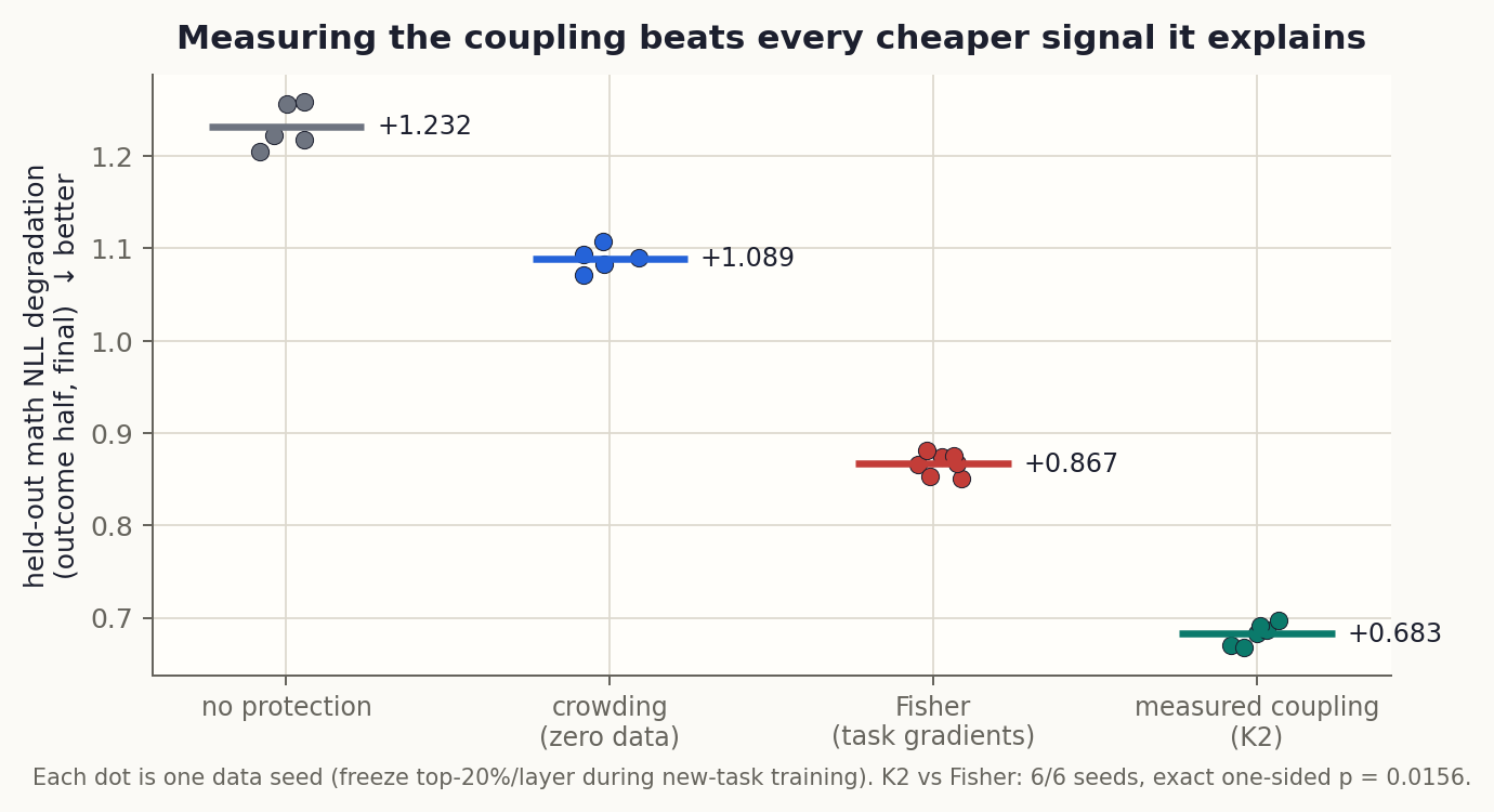
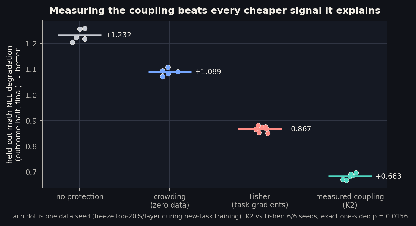
K2 beats crowding by -0.40 NLL and beats Fisher by -0.183 on every one of six seeds (exact one-sided p = 0.0156). The registered “strong result” band was merely matching Fisher; the data went past it. This is the strongest retention selector observed anywhere in this program, and it overlaps the crowding mask at only 0.32, so it is not crowding in disguise.
One fairness note, registered up front: K2 uses information Fisher does not have (that one unprotected B-run). But Suspect 3 already showed that update information alone is the worst selector in the program. Raw movement fails; movement weighted by curvature wins. The curvature weighting, not the data access, is what converts a B-run into the best mask.
Exhibit D: the value is off-diagonal, specifically
The remaining skeptical reading: maybe K2-high neurons are just fragile in every measurable way, and “off-diagonal” is along for the ride. Our first attempt at this control was itself caught by an adversarial audit: the matched sets turned out unbalanced on exact self-curvature and first-order alignment, so we relabeled that result and registered a stricter design with a stop-if-confounded gate.
Version 2 uses a near-exact diagonal estimator (agreement with exact self-curvature: rho 0.993) and builds three sets of 28,443 neurons matched on crowding, self-curvature, first-order alignment, Fisher, and movement, with a post-construction audit on exact quantities. The audit passed with the balance tilting slightly against the hypothesis (the high set’s self-curvature is 0.84x the low set’s). Then the causal test: restore each set to its pre-B values inside the damaged model and measure how much math returns.
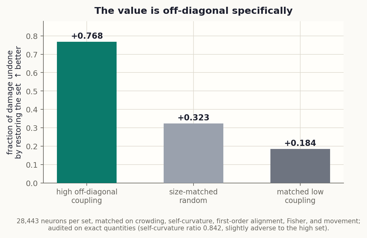
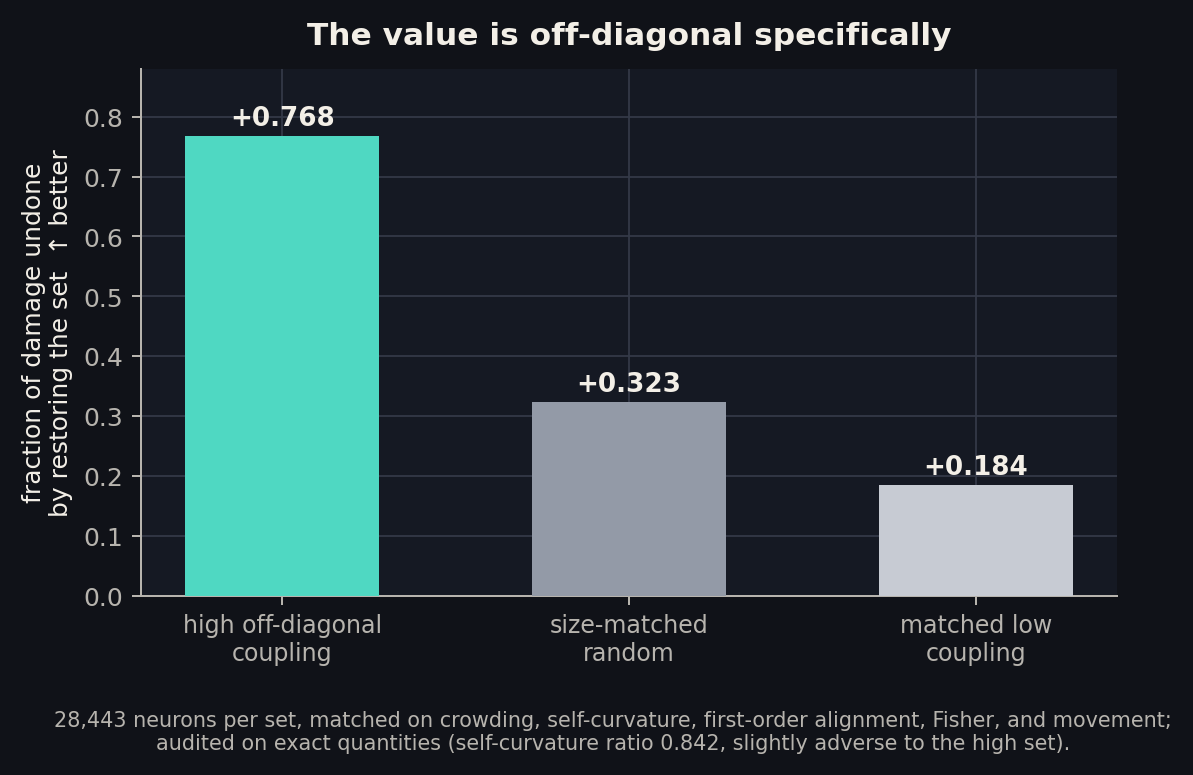
High-coupling neurons undo +0.768 of the damage. Their matched-on-everything-else low-coupling twins undo +0.184, less than a random set (+0.323). With every diagonal explanation held fixed and audited, the off-diagonal information alone separates recovery by +0.58. This is the finding the whole case rests on, and it survived the audit that killed its first version.
Two smaller pieces round out the picture. The neuron behaves as the natural unit: freezing its three weight matrices contributes protection almost exactly additively (shares 0.39 + 0.13 + 0.44, summing to 0.96), with no single interface acting as the mechanism’s home. And nothing here says forgetting is only off-diagonal; self-curvature is real, which is why Fisher is a strong selector. The claim is that the cross terms carry protection-relevant information that no diagonal signal contains, and that crowding is a free estimate of where those cross terms concentrate.
The confession doubles as a prediction
A good mechanism should tell you where it stops working. This one does.
Curvature in the optimizer’s coordinates is not a property of the abstract function the network computes. You can rescale a SwiGLU neuron (multiply its input row by a power of two, divide its output column by the same factor) and the network’s outputs do not change at all; with power-of-two factors the logits are bitwise identical. But the curvature account says the damage process should change, because the rescaling scales one damage pathway’s curvature by \alpha^2 and the other’s by \alpha^{-2}.
So we ran the final registered experiment as a self-test: if protection value is invariant under these function-preserving rescalings, the curvature account is wrong. It is not invariant. Rescaling the protected neurons by 4 or by 1/4 raises protection value by +163% and +99%; a global random rescale swings it by -126% (mostly by stalling learning: Adam’s per-parameter state is calibrated to the old scales). All three land far outside the registered +-25% invariance band, in the direction the algebra points.
The scope condition, stated plainly: crowding’s protection value is a joint property of the computation’s geometry and the optimizer’s coordinates, not of the function alone. Any deployment claim must hold the parameterization fixed. Real fine-tuning does exactly that, so the ledger applies where it is used; but nobody should carry these numbers across a reparameterization.
The causal chain is established in one primary regime: TinyLlama-1.1B, one math-to-code curriculum, 20% freezing budget, neuron granularity. The curvature object is the Gauss-Newton form (concordance with the full Hessian +0.67 on large entries; indefiniteness of the true Hessian documented). Crowding tracks within-layer coupling load (+0.32) but not the global cross-layer version (+0.18, a registered miss). The K2-versus-crowding paired comparison sits at the n = 4 exact-test floor (p = 0.0625); K2-versus-Fisher is the conventionally significant one (n = 6, p = 0.0156). On Qwen2.5-1.5B under a healthy validated protocol, total forgetting is 0.003 NLL, so there is nothing to dissect there; the aggressive-protocol Qwen results are scoped to that regime. “Polarity has no effect” means no detected effect. All amendments, gate stops, and the confounded first isolation control are disclosed in the preregistration trail.
The ledger, upgraded
Where does this leave the practical picture from Paper 1?
The two-signal ledger (weights as a structural prior, a small activation capture as calibration) turns out to have been approximating the two factors of off-diagonal curvature all along: the geometry clock and the usage clock. That reframe explains the program’s stubborn observations in one stroke. Why does zero-data crowding protect? It reads the geometry factor. Why does it protect while disagreeing with Fisher? Fisher is diagonal; the information is in the cross terms. Why did every co-firing test come up null? The co-activation-gated pathway carries 3% of the coupling. And why is protection value fragile under reparameterization? Because curvature is.
It also hands the next project its target. K2, the best selector we have ever measured, costs a full sacrificial training run. The registered follow-up question is a ladder: how close can you get to K2’s value with zero lookahead (a block-coherence ledger built from the weight file), or with 1, 4, or 16 early microbatches of the new task? The decomposition already tells us where to look: read-side co-response against the write-vector Gram matrix, not raw firing statistics. That allocator, a capacity ledger that knows what the next task is about to break before it breaks it, is Paper 3.
The earlier post ended by admitting that why crowding helps at all remained open. It is no longer open. Crowding helps because it is the visible half of the quantity that forgetting actually uses: the off-diagonal curvature that couples a neuron’s fate to its neighbors’. The weights were never a complete ledger. But on this question they were telling the truth, and now we know which truth.